Contact probability P(s)

Identical to its reference in the validationThe expected contact by separation, as cooltools’ expected_cis computes it (Open2C 2024). doi:10.1371/journal.pcbi.1012067

In the app

Analysis panel, under 2D tasks: Contact probability P(s)

Command

chromosomix expected

Reads

A contact map

Also known as

P(s), Ps, decay, distance, scaling, expected, slope

P(s), how contact falls with the distance between two loci along the sequence, is the first curve to draw of any contact map; its log-log slope shows a shoulder or a plateau the curve hides. Use it to compare libraries, conditions or organisms on one axis. The 4C profile, the compartments, the inter-arm alignment and the pileups each compute their own expected, so this task’s settings change none of them.

Running it

Open a contact map, choose Contact probability P(s) in the 2D tasks card of the Analysis panel, and press run. With scope on chromosome, the default, there is one curve per ticked sequence; whole genome pools every sequence into one.

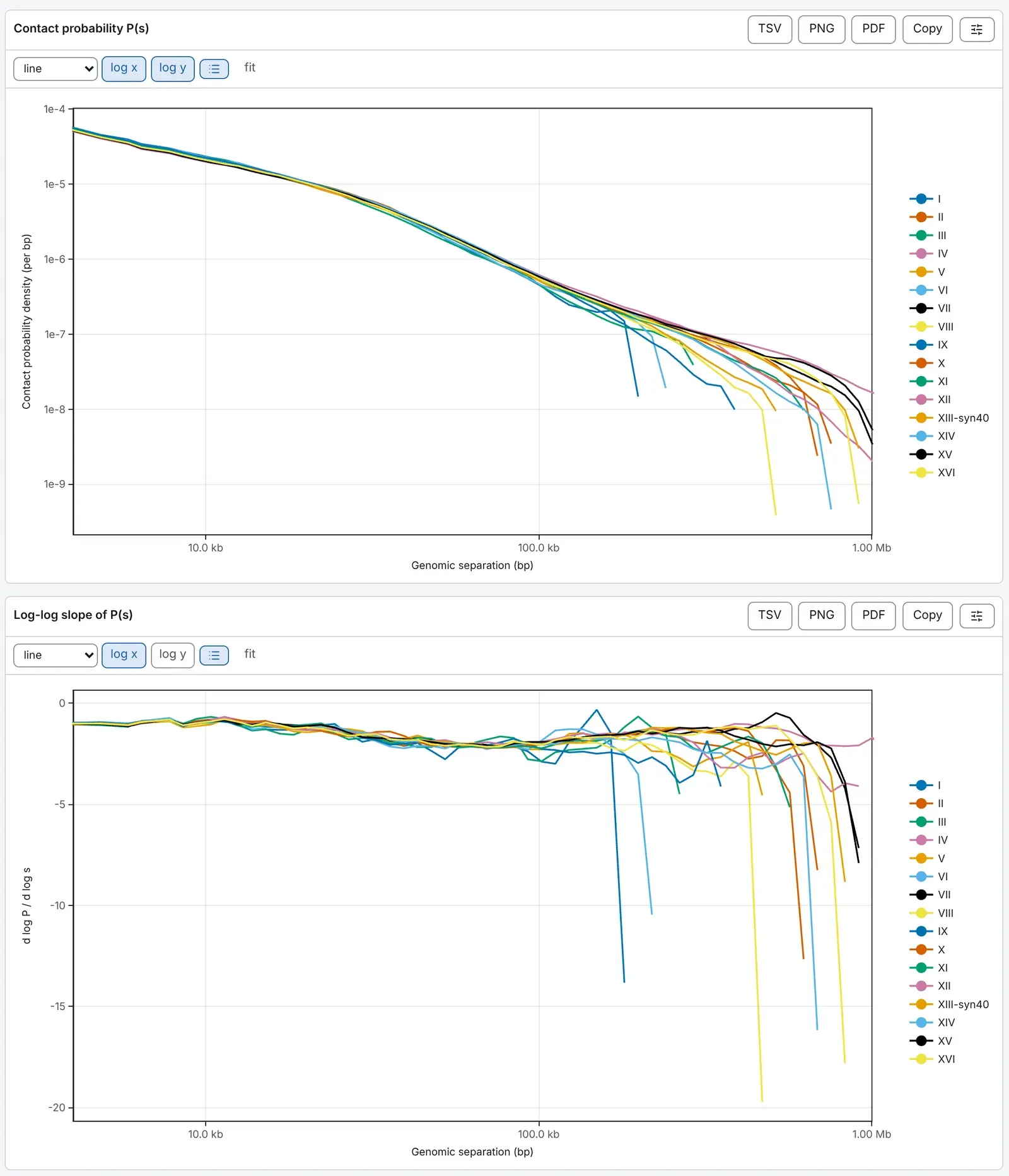
The drawer shows Contact probability P(s), a line per sequence, over Log-log slope of P(s), on logarithmic axes. Both open on 4 kb to 1 Mb, past the ligation artefacts and inside the shortest chromosome; the curve runs further, and fit shows all of it.

The same run from a shell:

chromosomix expected <map> [--<parameter> <value> …] --out <dir>

The expected, cooltools’ quantity, pooled over the whole genome:

chromosomix expected sample.mcool::/resolutions/1000 --quantity expected --scope file --out results/

Parameters

quantity matters, because two things are called P(s). probability density, the default, is the share of all cis contacts at each separation, per base pair, as HiContacts’ distanceLaw reports it. expected (cooltools) is the mean contact per pair of bins that far apart, as cooltools expected-cis reports it, and what most published scaling exponents use. minimum separation leaves out the diagonal and the one beside it by default, as cooltools does: they hold self-ligation and unligated fragments. log bins per step trades a smooth tail against a detailed shoulder.

Parameter	Takes	Default	What it does
scope--scope <value>	contig or file	contig	contig — one curve per sequence; file — every sequence pooled into one curve.
sequences--sequences <name,…>	sequence names, comma-separated	Every sequence of the file when left out.	—
quantity--quantity <value>	density or expected	density	density — share of all cis contacts, per base pair. HiContacts' norm_p; expected — mean contact per pair of bins that far apart. What cooltools expected-cis reports.
log bins per step--factor <n>	a number, 1.01 to 2	1.1	Each separation bin is this many times wider than the last.
minimum separation--minSeparation <n>	a whole number, at least 0, in bins	2	Drops the near-diagonal, where unligated fragments dominate.
log-log slope--derivative / --no-derivative	on or off	on	The shoulder and the plateau are visible there and not on the curve.
use balancing weights--no-balance	a switch	On wherever the file carries balancing weights; --no-balance reads the raw counts.	—

What it writes

• curve: a curve: TSV

On the command line every file goes into --out as <file stem>.expected.<output>.<ext>, and each TSV opens with # lines naming the build, the file and every parameter that produced it.

Reading the result

The curve is straight on the log-log axes wherever contact falls as a power of the separation. The two quantities agree at short separations and part near the length of the longest sequence: on the yeast demo map they are within 1 % below 10 kb, 13 % apart at 100 kb and a factor of fifty apart at 1.2 Mb, while on a mammalian map they agree over every separation anybody fits. Compare curves of one quantity, and say which a figure shows.

The slope, d log P / d log s, is the local exponent of the decay. Towards the length of the longest sequence each point rests on fewer pairs of bins, and both figures grow noisy.

What to watch for

• The density is not quite HiContacts’ on a matrix. HiContacts divides each logarithmic bin by its nominal width, which on a 1 kb map puts a sawtooth of a factor of two into the curve near 10 kb; chromosomix divides by the separation the bin actually covers. Past about 50 kb at 1 kb bins the two agree.
• The four read orientations are drawn by Pairs QC, from a .pairs.
• Counts, not another score. On a map drawn from another score column, a pass over the whole pixel table reads the stored counts, and the run says so; a run over one sequence measures that column.