Tracks and features

Dropped on a map, a track is drawn along any of the map’s four edges; opened with no map, it opens the 1D browser over its genome (The genome browser). Each track is a row of the Annotations panel’s Tracks card, whose Load a track zone takes a drop or a click.

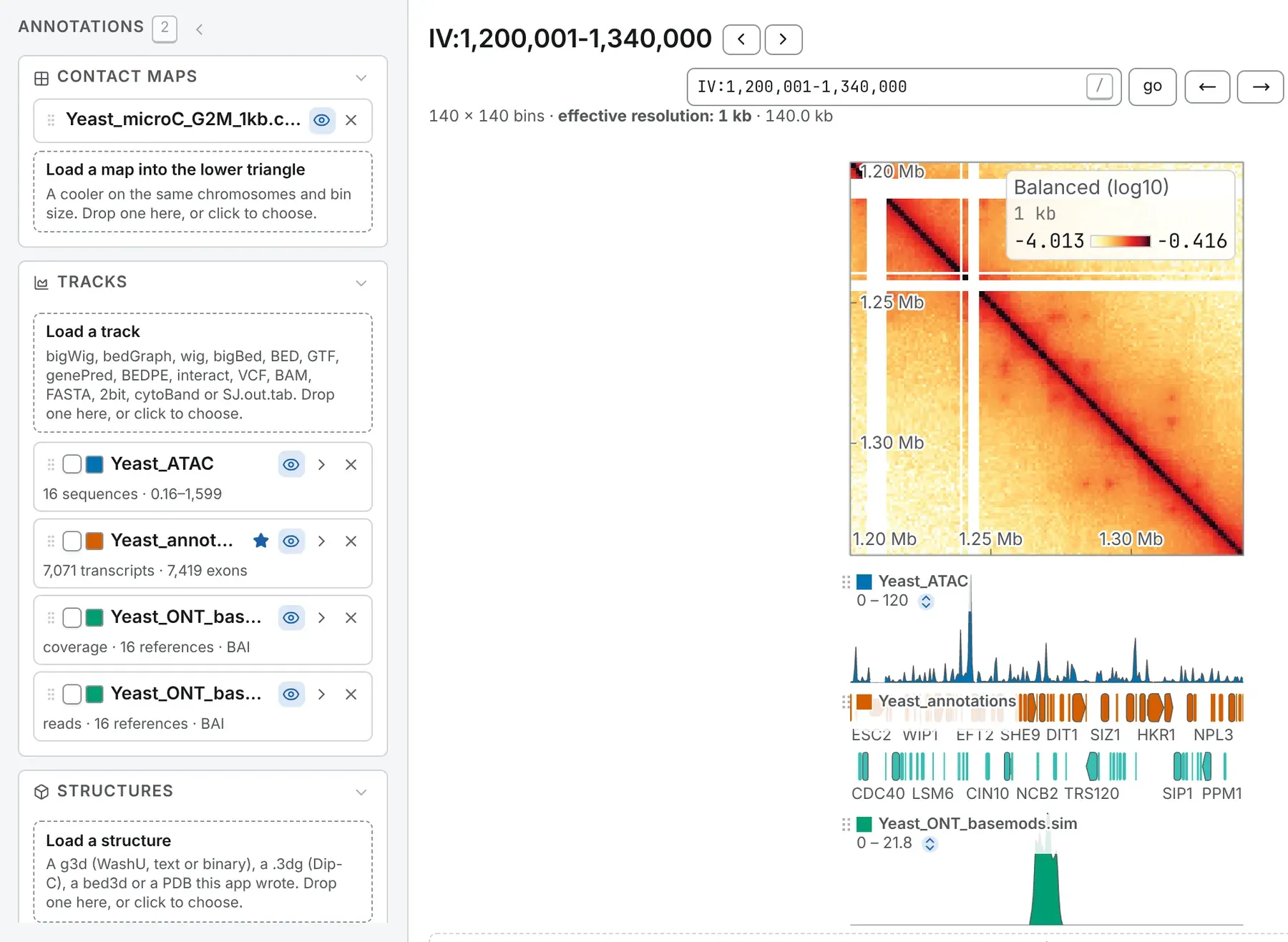
Sequence names are matched to the map’s even when spelled differently (chr1 against 1), and the row says when some do not match: 10 of 16 sequences matched; nothing is drawn on XI, XII, …. Pairs of loci are on Interactions; FASTA and .2bit on Reference sequences.

Signal: bigWig, bedGraph and wig

A bigWig, a bedGraph (exactly four columns, the fourth a number, or a track type= line) or a wig (fixedStep or variableStep lines, 1-based) draws as a value track with its own limits, colour and style, and can share an axis with others. A bedGraph or a wig is read whole.

Intervals: BED and bigBed

A BED of 3, 4, 5, 6, 9 or 12 columns, a narrowPeak, broadPeak or gappedPeak, or a headed table whose first three columns are a sequence, a start and an end opens as features beside the map, never on it. A BED12’s blocks are drawn as exons, its thick span thicker.

A bigBed is read whole, and cut off, with a note, past a million intervals. One whose schema says bigGenePred, bigBarChart, bigMethyl or bigInteract is read as that.

Gene models: GTF, GFF3 and genePred

GTF and GFF3 are read as transcripts from their exon and CDS rows, the coding span thick and the untranslated ends thin. A bacterial GFF3 from Prokka, Bakta or DFAST, whose rows name no parent, is read a feature per row, under its locus_tag and gene symbol.

genePred, genePredExt and refFlat open as the same gene models, with or without a leading bin column, and so does a bigGenePred. With several gene models loaded, the star on a row marks the one the locus box searches for gene names.

Called variants: VCF

A VCF opens as a lane of called variants: a substitution in the colour of the base it changes to; an insertion, a deletion or a symbolic allele (<DEL>, <DUP>) in grey, as wide as it is, from INFO/END or INFO/SVLEN. Click a variant for its card.

• With ##contig lines in its header, it opens the 1D browser on its own chromosomes, at their exact lengths.
• Samples are counted, not drawn: 1,284 variants · 2,504 samples not drawn.
• It is read into memory, so one human sample’s whole-genome calls are too large; split by chromosome, they open. BCF is not read: bcftools view writes a VCF.

Reads: BAM

A BAM opens as two rows:

• the depth row, under the file’s name: mean depth, a deletion counted as covered and a skipped intron not, secondary and supplementary alignments left out, duplicates kept unless you switch on hide duplicates;
• the reads row, name · reads, in the 1D browser only: the pile of reads.

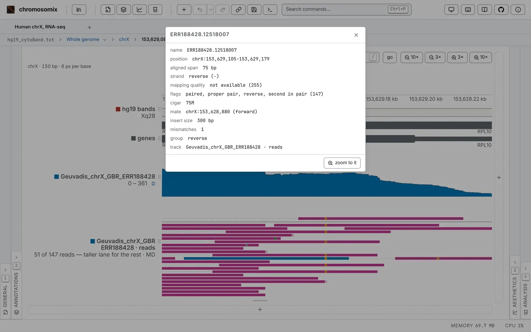
min MAPQ and hide duplicates apply to both rows; the colouring, the layout of pairs and split reads to the pile. Mismatches are coloured from the reads’ MD or =/X codes, or from a FASTA open in the tab; base modifications from the MM and ML tags (colour by → base modification on the pile, % modified on the depth row). A spliced library’s skipped introns are drawn as arcs over the depth (junction arcs, from two reads by default).

Without a .bai or .csi, the reads are found by searching the sorted file, a window of up to 4 Mb at a time (reads located by search). A window too deep to read, or a pile over too wide a window, draws nothing and says why: 12.4 MB of reads — zoom in.

A BAM must be sorted by coordinate: one sorted by read name, or a Hi-C pipeline’s alignment file, is refused with the fix:

samtools sort -o sorted.bam reads.bam
samtools index sorted.bam

For Hi-C, open the .pairs or the contact map instead. CRAM is not read: convert it with samtools view -b.

Methylation: bedMethyl and bigMethyl

A bedMethyl (from modkit pileup, or ENCODE’s older WGBS layout) or a bigMethyl opens as percentage modified per base, on a 0 to 100 axis at first. Where several modifications cover the same bases, the commonest is drawn, and the lane’s summary lists every code (m 5mC, h 5hmC, a 6mA…) with its count of rows. A row with no reads is left out, not drawn as 0 %.

Charts: barChart and bigBarChart

A barChart gives each feature a vector of values: a small bar chart where there is room, otherwise one box in its top category’s colour and height. Names and colours come from the track line (barChartBars, barChartColors); a bigBarChart opened alone has none, so its categories are numbered.

Charts on a lane share one ceiling, the file’s maxLimit or its largest value. scale each chart scales each to its own tallest bar; typed limits fix the axis, to compare two files. Click a feature for its whole chart.

Ideograms: cytoBand

A cytoBand or cytoBandIdeo draws each chromosome’s Giemsa bands. The line under the lane names the bands in view (Xq27.3 – q28), a click names one (Xq28), and the locus box finds bands by name. A cytoBand that tiles every chromosome declares the genome: UCSC’s hg19_cytoBand.txt alone opens the browser over hg19.

Splice junctions

Junctions are drawn as a sashimi plot’s arcs, each labelled with its read count, from three files:

File	Written by	Recognised by
SJ.out.tab	STAR	its nine integer columns
a junctions BED12	regtools, TopHat, Portcullis	junc or sj in its name, a TopHat track line, or JUNC… row names
.junc	leafcutter	its name

Each junction’s card shows the file’s other columns, which can also colour the lane: colour by annotated to see novel splicing. Junctions on both strands split the lane, forward above, reverse below. The lane’s lower limit filters, as a sashimi plot’s minimum junction coverage does. A spliced BAM draws its own arcs (above).

Lengths: chrom.sizes

A chrom.sizes (or a .genome file: a name and a length per line) declares a genome. Opened alone, it starts the 1D browser on those sequences. Dropped on a browser whose lengths were guessed from a feature file (inferred (rounded up) on the Genome card), it gives the real ones.

Reading part of a large text file

Text formats are read whole, unless bgzipped and indexed with tabix: then only the sequences the map holds are read.

sort -k1,1 -k2,2n peaks.bed | bgzip > peaks.bed.gz
tabix -p bed peaks.bed.gz

Keep the .tbi beside the file, drop the two together, or name it with #index=<address>. Without a usable index, or where it would save less than a fifth of the file, the whole file is read. A browser holds little more than half a gigabyte of text: index a larger file, or split it by chromosome.

The file’s own columns

A feature lane is coloured by strand at first. Its colour by offers the file’s other columns (a GTF’s biotype, a VCF’s QUAL, a BED’s name…) as categories, commonest first, or, for numbers, as a colour ramp over the whole file’s range. Names exactly A and B take the compartments’ red and blue.

The Metadata annotations card, folded at the foot of the Annotations panel, offers a cooler’s own columns, such as its balancing weight, where the view can show them. Pick one and press add to draw it as a lane, numbers as bars and labels as runs of colour; its row exports it as a TSV.