Your first map

A first session on public data; you need a recent browser and a network connection. The map is in situ Hi-C of K562 cells from the 4D Nucleome project (4DN), 4DNESC23ZYOF (Belaghzal et al. 2021): about 187 million contacts on GRCh38, in a 1.9 GB .mcool read by range. The guided tutorial plays the same session in the app.

Open the app

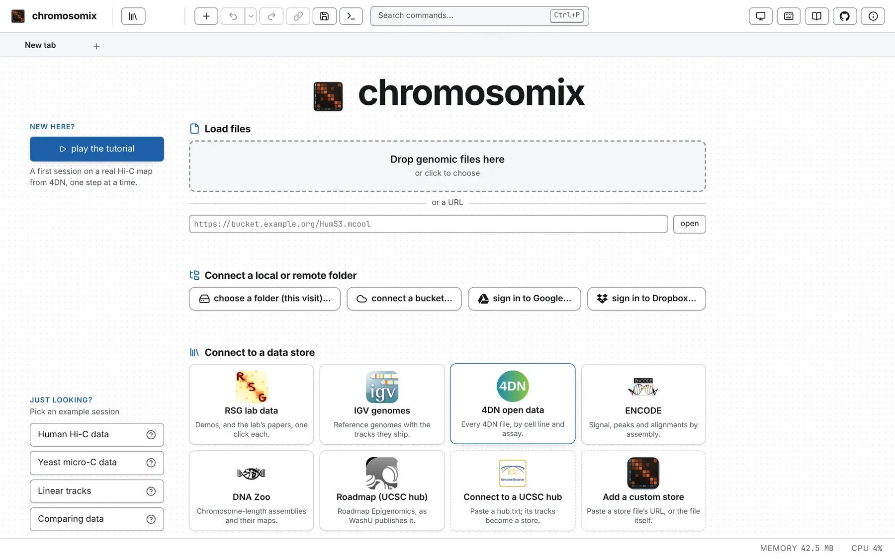
Go to https://chromosomix.app/. The landing page opens files from your disk or a URL (Load files), a folder, bucket, Google Drive or Dropbox (Connect a local or remote folder), or a catalogue of published data (Connect to a data store). Under Just looking?, Human Hi-C data opens K562 at the MYC locus with its tracks; each example’s ? says what it opens.

The landing page: play the tutorial under New here?, Load files with its drop area and URL box, the four buttons that connect a folder, a bucket, Google Drive or Dropbox, and the data store tiles with the pointer on 4DN open data.

Open a map from the 4DN store

Under Connect to a data store, press 4DN open data. The store drawer opens.
In its search box, type 4DNESC23ZYOF.
On the set’s heading, press open with its tracks. The map opens with 4DN’s own compartment eigenvector (E1), insulation score and boundaries.

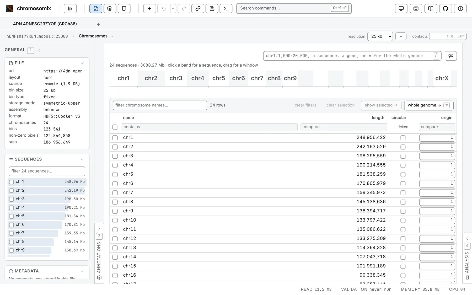
It opens on the Chromosomes table, beside the General panel, which describes the file.

The Chromosomes table of 4DN’s K562 map, a row per chromosome with its length, beside the General panel, whose File card gives its bin size, 25 kb as it opens, and a sum of 186,956,649 contacts, and whose Sequences card lists its chromosomes.

Pick a resolution and open a chromosome

After resolution, at the end of the bar above the table, choose 250 kb: a dropdown here, a slider on a file with nine bin sizes or fewer.
In the Chromosomes table, press chr15.

The blank square at the start is the short arm, with no unique sequence for reads to map to; the checkerboard off the diagonal is the long arm’s compartments.

Move around

Drag pans, the wheel or a pinch zooms, double-click fits the picture. After a click on the map, the arrow keys pan it; 0 fits it from anywhere.
To open a stretch rather than enlarge it, hold ⌥ Option (Alt on Windows and Linux) and drag a box across it; add ⇧ Shift to keep it on the diagonal.
Or type a place, chr15:30,000,001-60,000,000, and press go. Coordinates are 1-based and inclusive, as in IGV and UCSC.
Beside go, two arrows move half a window, and 10×, 3×, 3×, 10× zoom out or in.
The trail above the map (the file, Chromosomes, chr15, the window) and the header’s back button take you back up; in a window of one chromosome, a click on the map opens it whole.

Moving around has every gesture and key.

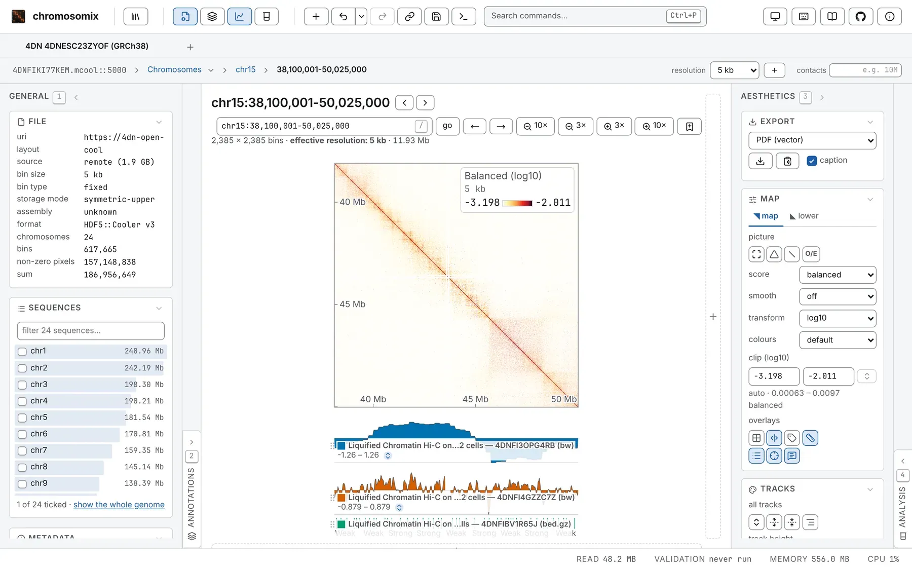
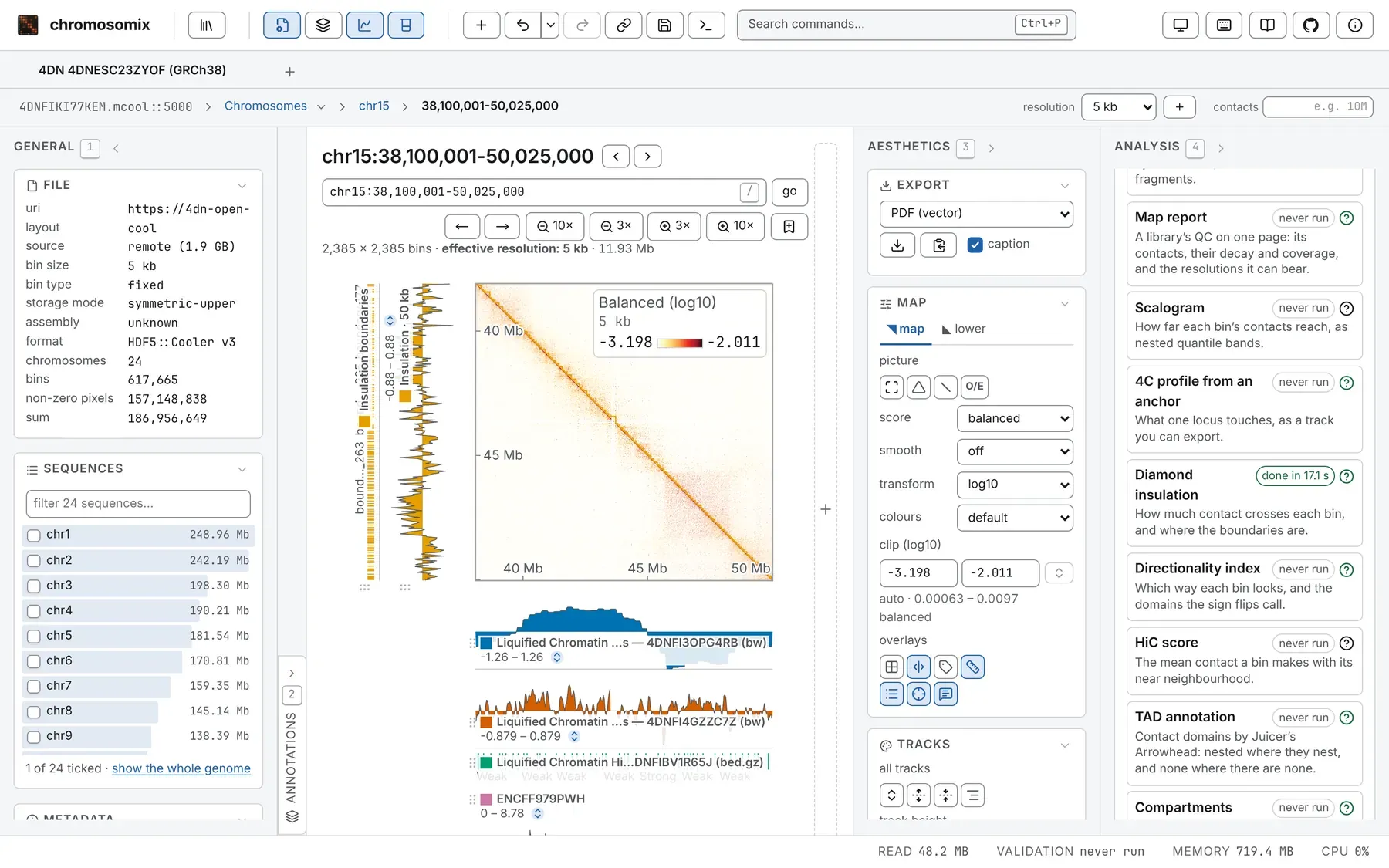
Change the resolution

Open chr15 from 30 to 60 Mb and choose 5 kb. Closer in, at chr15:38,100,001-50,025,000, the squares along the diagonal are domains, mostly nested, and the dots at their corners are loops.

A window with more bins than the picture has room for is drawn coarser, at the effective resolution given under the title. - and + step coarser or finer.

chr15,100,001-50,025,000 at 5 kb, balanced on a log10 scale, with 4DN’s compartment eigenvector, insulation score and boundaries drawn under the map.

Change the normalisation

On the Map card of the Aesthetics panel:

score: this file opens balanced, from its own weights; counts is the raw counts, coverage bias included. VC, VC √ and ICE are computed in the page; expected is the decay with distance alone; correlation, the plaid compartments are called from.
O/E (E) divides each pixel by what its distance predicts: red is more contact than that, blue less.
smooth averages neighbours: 3 × 3 evens out the sparse pixels of 5 kb.
transform, colours and the two clip boxes set the colour scale.

O/E and smoothing change the picture, not what an analysis reads. Reading a contact map explains each score.

Add a track

To add ENCODE’s CTCF ChIP-seq of K562, press + in the header (Add a file to this tab), paste this address under or a URL, and press open:

https://encode-public.s3.amazonaws.com/2020/09/26/85161a5a-d6b5-49d2-bc0a-db0b217ff0d5/ENCFF979PWH.bigWig

It is drawn under the map; its row on the Tracks card of the Annotations panel (2) sets its colour, height, range and edge. A file from your disk can be dropped on the window, on an edge of the map or on Load a track (Tracks and features).

Run an analysis: insulation

Insulation scores how much contact crosses each bin; its dips are domain boundaries.

Open the Analysis panel (4): 2D tasks read the map, 3D tasks model it, 1D tasks read tracks.
Under 2D tasks, press Diamond insulation. Its drawer opens.
It runs on every chromosome by default: in its list of sequences, press none, then tick chr15.
Keep the other defaults (a window of 10 bins, 50 kb at 5 kb) and press run.

The row says running, then done, while the map stays live. Close the drawer (Esc) to see the score, its boundaries and its domains, each a row of the Tracks card; the score’s row saves it as a bigWig.

chr15,100,001-50,025,000 at 5 kb after Diamond insulation, its row on the Analysis panel saying done: the computed insulation score and the boundaries it called drawn left of the map, the domains as corners along the diagonal, and 4DN’s tracks and ENCODE’s CTCF signal under the map.

The console (Ctrl and the key left of 1, Control on a Mac too) shows the run as the chromosomix command that repeats it. Diamond insulation explains the settings and the result.

Press Share this tab as a link in the header: the Share this tab dialog opens with the link copied. It holds the whole tab — view, tracks, marks, bookmarks — so no server keeps it and it never expires; as these files are public, anyone who opens it sees what you see. A computed track comes back with recompute.

shorten with is.gd sends the link, file address included, to that third-party service. Save every tab as a file (Ctrl+S, ⌘S on a Mac) keeps every tab (Sessions, workspaces and links).

Opening files: your own files.
Maps side by side: several maps at once.
A tour of the window: the rest of the screen.
Analyses: the other tasks.

Documentation of chromosomix v0.20.0 · built from 40ec1ec · source