The genome browser

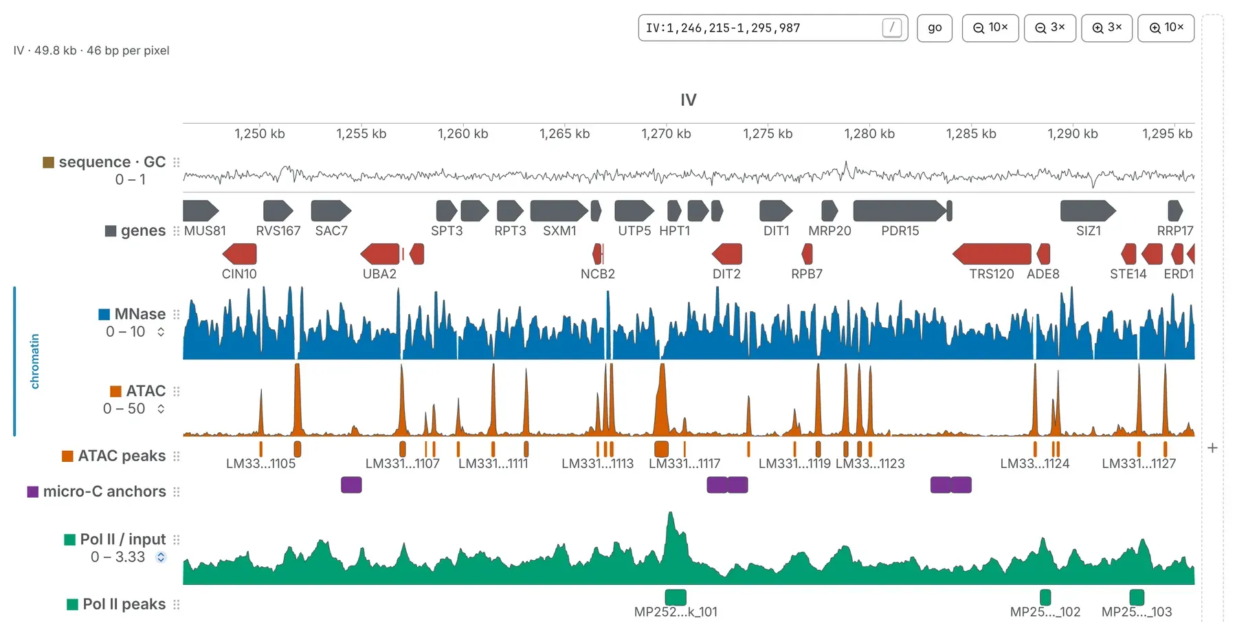
The genome browser stacks tracks along one axis, every sequence laid end to end. A tab shows it when it holds a genome but no map; beside a map, the same tracks line the map’s edges.

Opening it

Open a chrom.sizes, a FASTA or .2bit, a bigWig, a bigBed, a BAM, a VCF, a cytoBand or a feature file with no map open, and the tab becomes a browser over its genome (Opening files), as it does for a 3D structure. A feature file gives only lower bounds for the lengths, and the summary line ends lengths inferred (rounded up): drop a chrom.sizes or a bigWig on the tab for the real ones.

With a map open, v cycles through the map with its tracks, the tracks alone and the map alone. On the Contact maps card, the map row’s eye hides the map, and its × closes it, keeping its genome, tracks and marks in the browser. Drop a .cool on the browser and it becomes the tab’s map.

Moving along the genome

The locus box, go, the zoom steps and the gestures, from drag and scroll to ⌥ Option-drag and < >, work as on a map (Moving around). In the browser, also:

• the box takes a single position, IV:450000, for a window around it, and * for the whole genome;
• drag along the ruler to zoom to a stretch, click a sequence’s name on it to go there, and double-click for the whole genome;
• a drag across two sequences zooms but copies nothing;
• once you have clicked the tracks, the arrow keys pan, - and + zoom like the 3× buttons, and 0 shows the whole genome.

The card beside the pointer reads every track at that position. The address holds the window as locus=, with view=browser (Link keys), so a link you copy opens where you are. Tick sequences on the Sequences card (General panel) to make the axis those alone; show the whole genome clears the ticks.

Lanes and tracks

A track is a file you loaded, or a task’s result, with its settings; a lane is a place where it is drawn. Each track is a row of the Tracks card (Annotations panel), in lane order, with an eye that hides it, a chevron for its settings, a × that removes it and a grip to reorder. Drop a file on the card, or on its Load a track zone, to add one (Tracks and features); a genome published with tracks has a button that loads them all.

On a lane:

• click the colour chip to recolour the track, and the name to rename it;
• click either end of the value range to type a bound, which turns autoscale off; ⇅ turns it back on, and Tab moves to the next bound, then the next track;
• drag the lane’s lower border to resize it, and its handle, in the margin, to move it;
• drag across the lane, or scroll over it with ⌘ held (Alt on Windows and Linux), to move its ceiling;
• right-click it for Copy this (the lane as a PNG), Colour…, Range (Auto, or fixed), Hide, Remove and Duplicate; on a feature, the menu starts with About it…, Zoom to it, Copy its name and Copy its position.

The bar under the last lane resizes every track in proportion: drag it or step it with the arrow keys, and double-click it to fill the window; Esc during a drag undoes it. On the Tracks card of the Aesthetics panel, all tracks autoscales every lane (y), gives them one height that fills the room (h) or shrinks them to the shortest, and track height sets one height for all, from 12 to 400 pixels.

How a track is drawn

A track of values — a bigWig, bedGraph, wig or bedMethyl, a BAM’s depth — is drawn in a style:

Style	Draws
area, line, bar	the value as a filled area, a line, or a bar for each value
points	a dot for each value: a Manhattan plot, for p-values or sparse scores
heatmap	the value as a colour, costing no height; several in one lane stack, each with its colours
ribbon	the band between this track and the next in its lane, for a set of quantiles

scale is linear or log₂, where a value at or below zero leaves a gap. limits sets the lane’s foot, an optional centre the bars grow from (1 for a ratio) and its head; a head below the foot turns the track upside down, as flip does.

A track of features — genes, peaks, a BED, bigBed or VCF — draws blocks, or transcripts as exons on a thin line, thick where they code. Zoomed far out, the lane counts them.

• rows: expanded (the default, with names and the strands apart), squished (thin rows, no names) or collapsed (one row).
• colour by: strand (the track’s colour forward, a turned hue reverse, grey for none) or any column, such as a GTF’s biotype, with a key under the picker.
• point strands ends each stranded feature in a point.

The Annotations panel

Besides Contact maps, Structures and Tracks, the Annotations panel holds Manual annotations, whose buttons beside the browser read pick on track and draw on track: a mark lands on the diagonal, and a map opened later shows it (Annotations and bookmarks). With a map open, Metadata annotations draws the map file’s own columns, such as a cooler’s balancing weight, as tracks.

Editing several tracks at once

Tick two or more rows of the Tracks card (Shift-click for a range) and a box above the list offers hide or show, remove, clear, and the settings — colour, height, style, scale, flip, limits, group, location — for every ticked track they apply to, reading mixed where they differ. With two ticked, combine… makes a track of their ratio or difference, worked out on their own intervals.

Groups

A group is a set of tracks read on one scale, such as replicates. Tick their rows and choose a group in the box above the list, or set group in a track’s settings, where new group… makes one. The Groups card (Aesthetics panel) switches each group between one lane and a lane each, and between one pair of limits, which makes the members comparable, and one each; two buttons give every member the tallest’s or the shortest’s height. A group’s eye hides its members, and the × beside one takes it out.

Reads from a BAM

A BAM opens as two rows of the Tracks card: its depth, the mean coverage per bin, a track like any other; and … · reads, the reads themselves, drawn only in the browser. Each row is resized, hidden or closed on its own. min MAPQ and hide duplicates (off by default) set the reads both rows count. Secondary and supplementary alignments never count, nor does a spliced read’s intron; junction arcs draws the introns over the depth, as a sashimi plot does.

On the reads row:

• draw as: pairs (the default: both ends of a fragment on one row, joined by a dotted thread), fragments (one bar each) or reads (every record alone, for a single-end library);
• colour by: strand, pair (proper or discordant), insert size, mate (where the mate went), mapq, base modification or none;
• split reads outlines the other pieces of a read split across a breakpoint, never counting them;
• click a read for its flags, CIGAR, clips, mate and insert size.

base modification reads the MM and ML tags that nanopore and PacBio basecallers write: red where a call is modified, blue where not, fainter the less sure. Under the picker, choose the modification and how sure a call must be. On the depth row, % modified draws the share of modified calls at each base or bin. Mismatches with the reference are marked on the reads and, with the genome’s FASTA open, on the depth row too, once more than a fifth of a bin disagrees.

A BAM has no zoomed-out summary, so too wide a window draws nothing until you zoom in. For a whole chromosome’s coverage, a bigWig made from the BAM is faster (Tracks and features).

The sequence lane

A FASTA or .2bit gives the genome and a lane: the GC content per bin, then the bases once each has a pixel. Beside a map it is always the GC content.

• reading frames, in the lane’s settings, adds the six frames, +1 to +3 over −1 to −3: close in, each codon with its amino acid, starts green and stops red; further out, the starts and stops alone. Beside the switch, pick any of NCBI’s genetic codes (table 4 for a Mycoplasma).
• Copy sequence, on the lane’s right-click menu, copies the bases in view, keeping their case.
• Drag across the letters to select a stretch, and ⌘ C (Ctrl C) copies it, or its protein on a frame.

A FASTA over 64 MB, read a window at a time through its .fai, draws its GC content only in windows under 4 Mb (Reference sequences).

Tracks beside a map

Beside a contact map, tracks stack on its four edges. A track’s location, in its settings, has a mark for each edge, lit where the track is drawn; a track can be on several. Drag a file over the map and a strip lights along each edge, with on this map in the middle: let go on a strip for that edge. A lane dragged by its handle moves to another edge.

Lanes above and below the map grow up the page; on the left they grow away from the map, on the right towards it. On a lane’s right-click menu, Grow away from the map (or Grow towards the map) turns it over, and Draw it moves it to another edge. Pairs — a BEDPE, interact or longrange file — and called loops are drawn on the map as circles, or as arcs along an edge.

name column (u) moves the tracks’ names from over their lanes to beside them. In a deck each map has its own lanes.

A lane beside a map shares its axis: drag along it to pan the map, scroll to zoom, and Shift-drag to zoom the map to that stretch on the diagonal and copy its coordinates. A form that asks for a place, such as the 4C profile’s anchor, has a pick on map button: press it, and your next drag on a map names the place.

Circular sequences

Nothing in a .cool or a FASTA says a sequence is circular: tick its circular box in the Chromosomes table (the crumb after the file’s name, or c). Its origin, where replication starts, counted from 1, is the first base until you or the Origin and terminus task set another; type a position to move it, or empty it to go back. A declared sequence wears a ↻ on the Sequences card.

When a contact map first opens, its longest sequences are checked for contacts joining their two ends; those that look circular are ticked, and a banner says so. This only adds ticks, once per file. A genome opened as tracks has nothing to check: tick its circles yourself, and a map opened on it later takes them.

A tick makes P(s), insulation, the directionality index, the HiC score, the scalogram, compartments and the tasks read from the origin measure separation the short way round. Chromosight and the map’s own O/E, unless arms is on, do not, so a seam at the junction is not a feature of the data.

On the map, a window may be typed across the origin (chrom:2,900,000-100,000 on a 3 Mb circle), and ori on the Map card frames the circle with the origin in the middle. The declarations are kept with the file and in a saved workspace, not in a link.