Loop calling

Identical to its reference in the validationHiCCUPS (Rao et al. 2014), as cooltools.dots computes it. doi:10.1016/j.cell.2014.11.021

In the app

Analysis panel, under 2D tasks: Loop calling

Command

chromosomix loops

Reads

A contact map

Also known as

loops, dots, call loops, hiccups, peaks, cooltools dots

Loop calling answers where are the loops by testing every pixel of the map against four local backgrounds. Pattern detection finds loops by template matching instead; run both when it matters which loops you trust.

Running it

It needs a map that carries balancing weights; on a file with none the row waits, saying to run cooler balance on it. In the Analysis panel (4), choose Loop calling, tick the sequences, and press run. Each sequence is read as a band along its diagonal, out to furthest from the diagonal.

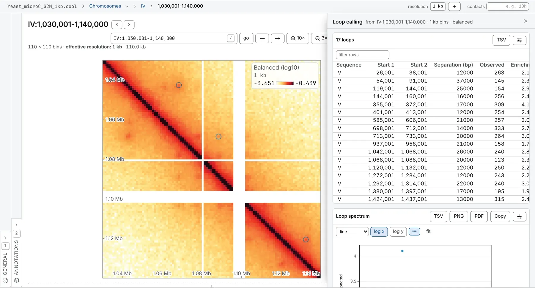
Called loops lands on the map as a ring round every loop: a row of the Tracks card in the Annotations panel, marked *, whose display can make it arcs (1D track). The notes give the kernel, the scan’s reach, and how many pixels and clusters passed. Pile the loops up with aggregate peak analysis to see them on average.

The same run from a shell:

chromosomix loops <map> [--<parameter> <value> …] --out <dir>

Parameters

The kernel is the one setting with no default. cooltools has kernels for bins of 4 to 28 kb: outer half-width 7 and inner half-width 4 from 4 kb, 5 and 2 from 8 kb, 3 and 1 from 18 kb. The boxes are filled from that for your map; outside it, as on a 1 kb yeast map, they are empty and the run is refused until you fill them.

Furthest from the diagonal and clustering radius start at 10 Mb and 20 kb in the map’s bins, and follow the resolution until you type your own.

Parameter	Takes	Default	What it does
General
sequences--sequences <name,…>	sequence names, comma-separated	Every sequence of the file when left out.	—
outer half-width--outer <n>	a whole number, 1 to 50, in bins	Worked out from the map's bin size when left out; 5 where there is no map.	W: how far the donut and the other three neighbourhoods reach from a pixel.
inner half-width--inner <n>	a whole number, 0 to 49, in bins	Worked out from the map's bin size when left out; 2 where there is no map.	P: the square about a pixel none of the four counts, a loop’s own size.
furthest from the diagonal--maxSeparation <n>	a whole number, at least 1, in bins	Worked out from the map's bin size when left out; 1000 where there is no map.	Loops whose anchors are farther apart are not looked for; 10 Mb unless changed.
use balancing weights--no-balance	a switch	On wherever the file carries balancing weights; --no-balance reads the raw counts.	—
Statistics
false discovery rate--fdr <n>	a number, 0.001 to 0.5	0.1	Benjamini–Hochberg, within each λ-chunk of pixels of a like local expected.
λ-chunks--lambdaBins <n>	a whole number, 40 to 50	40	Log-spaced chunks of local expected, each corrected on its own; 40 to 50 of them.
Clusters
clustering radius--clusteringRadius <n>	a number, at least 0, in bins	Worked out from the map's bin size when left out; 2 where there is no map.	Enriched pixels this close are one loop, at its brightest; 0 keeps every pixel, unfiltered.
enrichment filter--filter / --no-filter	on or off	on	1.5–2× over the four neighbourhoods, and a lone pixel only at q ≤ 0.02 summed over them.

What it writes

• intervals: a set of intervals: TSV, and BED (or BEDPE for pairs, or bed3d and PDB for a 3D model)
• curve: a curve: TSV
• table: a table: TSV

On the command line every file goes into --out as <file stem>.loops.<output>.<ext>, and each TSV opens with # lines naming the build, the file and every parameter that produced it.

Reading the result

How a pixel is called

Each pixel is compared with four neighbourhoods out to the outer half-width, less the inner half-width’s square about it: the donut around it, a vertical and a horizontal bar through it, and the square below and left of it. Each gives a locally adjusted expected, λ: the distance decay at the pixel, scaled by what the neighbourhood holds over what the decay predicts, in raw counts, so the pixel’s raw count is tested against a Poisson tail.

Pixels are grouped into λ-chunks of like expected, and Benjamini–Hochberg runs within each, kernel by kernel, at the false discovery rate. A pixel that passes in all four neighbourhoods is enriched, and enriched pixels within the clustering radius of each other are one loop, at its brightest pixel. The enrichment filter then keeps a loop at 1.5 times its vertical and horizontal expecteds, 1.75 times its donut and lower-left ones and twice one of those two, and a single-pixel cluster only where its four q-values sum to 0.02 or less.

The table and the loop set

A row per loop: Start 1 and Start 2, the bins of its anchors, and their Separation (bp); Observed, the raw contacts in the pixel; Enrichment, observed over the donut’s λ; the four λ, in raw counts; the four q-values; and Cluster, how many enriched pixels its cluster held. The loop set holds the same calls, each anchor one bin wide, scored by its enrichment, and saves as a BEDPE.

The loop spectrum

The Loop spectrum sets each loop’s enrichment against its anchors’ separation, with the median in log-spaced bands. A pileup averages separation away, so short-range loops and long-range noise make one plausible dot; here they come apart. Be wary of scores that fall steadily with separation, or pile up at the nearest separation the scan reaches.

Contacts needed, by λ-chunk

For each chunk, the count a pixel had to reach to pass, kernel by kernel, against the line where a pixel merely meets its expected. On a sparse map it shows thresholds nothing in the map could reach.

What to watch for

• Near the diagonal. The nearest pixel tested is twice the outer half-width plus two bins from the diagonal, and a bin the balancer dropped takes out the pixels within the outer half-width of it. The notes say how near the scan came.
• Band size. A sequence whose band would not fit is skipped and named: bring furthest from the diagonal down, or open a coarser resolution.
• Too bright for the chunks. A pixel whose expected is past the last λ-chunk stops the run, which says so: raise the λ-chunks, up to 50.
• Nothing passed. The run says so, and still draws the λ-chunk thresholds to show how far out of reach they were.

Compared with cooltools

Every default is that of the Python API’s dots(): a 10 Mb scan, a 20 kb clustering radius, an FDR of 0.1 and 40 λ-chunks. cooltools’ command line uses 2 Mb, 39 kb and 0.02, so give the same numbers to compare a cooltools dots run. In § 19 of the validation, on a mouse Hi-C map at 10 kb, it calls the same loops at the same pixels as cooltools.dots, with the same contacts, and expecteds and q-values that agree to the digits written.